
Forecasting - What is it? (Part 1)
Time Series Forecasting

Disclaimer: This post summarizes key insights and lessons from the Coursera course "Excel Skills for Business Forecasting Specialization" taught by Dr. Prashan S. M. Karunaratne, from Macquarie University. This summary is intended to provide an overview and encourage further learning. For a complete understanding, I recommend taking the course directly on Coursera.
Excel Time Series Models for Business Forecasting
Excel Regression Models for Business Forecasting
Judgmental Business Forecasting in Excel
Table of Contents
Something before we dive in
Forecasting is both an art and a science. It involves using historical data, statistical tools, and expert judgment to make informed predictions about the future. Whether you're in business, finance, or any other field that requires anticipating future trends, mastering the basics of forecasting can give you a significant edge.
Before we delve into the various forecasting methods and their applications, there is something important that should be noted first.
Types of Forecasting Methods
There are a number of classifications of forecast methods:
Qualitative vs Quantitative
Quantitative – the prediction is derived using some algorithm or mathematical technique based on quantitative data.
Qualitative – the prediction is based primarily on judgment or opinion.
Time Series vs Causal
Time Series – These are methods which rely on the past measurements of the variable of interest and no other variables, e.g.: moving average, exponential smoothing, decomposition, extrapolation…
Causal methods – where the prediction of the target series or variable is linked to other variables or time series, e.g.: regression, correlation and leading indicator methods.
The above classifications are not mutually exclusive. The forecaster needs to be aware of the appropriate method to match the forecast situation.
Data Source
Predictions and forecasts are based on relevant current and past data. The data sources can be classified into internal and external.
Internal sources come from within the organization, for example, sales data, employment records or customer profiles.
External sources come from outside the organization, for example, bureau statistics data, government agencies, or commercial data agencies.
Types of Data
A useful classification of data for forecasting is whether the data is time series data or cross-sectional data.
Time series data is a sequence of measurements on a single variable taken over specified successive intervals of time. For example: monthly interest rates, sales per week or tourist arrivals per month.
Cross-sectional data are measurements on a variable that are at one point in time but spread across the population. For example: tourism spending across different cities or production across different businesses in the country.
How does business forecasting work in a nutshell?
It's a three step process.
Step 1: Evaluation of the time series for historical patterns.
Step 2: Matching this observed pattern to irrelevant algorithm, the forecasting method.
Step 3: Projection of the algorithm into the future to produce our forecasts.
Discussed Concepts
Forecasting Methods: Forecasting involves producing models that accurately predict future data points (out-of-sample forecasts) rather than just fitting observed data (within-sample forecasts).
General vs. Sample Model: It's crucial to find a general model that explains and predicts both past and future samples. This model should capture the systematic components of the generating process, leading to accurate forecasts with unbiased predictions and reduced error variance.
Error Term: The error term in forecasting refers to the difference between actual data and forecasted data at each time point (residual). In a correctly specified model:
The error term should have a mean close to zero (assuming zero mean error).
Errors should be symmetrically distributed around zero without systematic patterns over time.
Errors should be uncorrelated over time, ensuring the model's reliability.
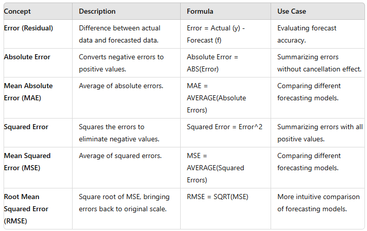
Accuracy Checks: To evaluate forecasting models, error functions are used, which mathematically summarize errors. Common error functions include:
Mean Absolute Error (MAE): Average of the absolute errors.
Mean Squared Error (MSE): Average of the squared errors. These functions help assess the model's performance by quantifying the deviation between actual and predicted values.
In this article, I want to look at three different models for forecasting:
Time Series Model
Regression Model
Judgmental Business Forecasting
Let’s start with the first one.
TIME SERIES MODEL OVERVIEW
Decision Tree
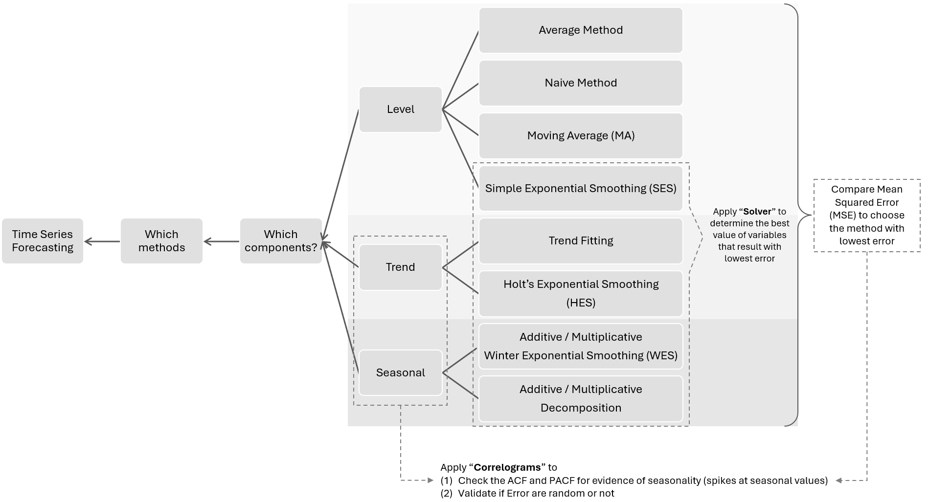
Component Types
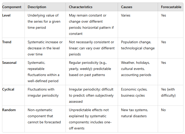
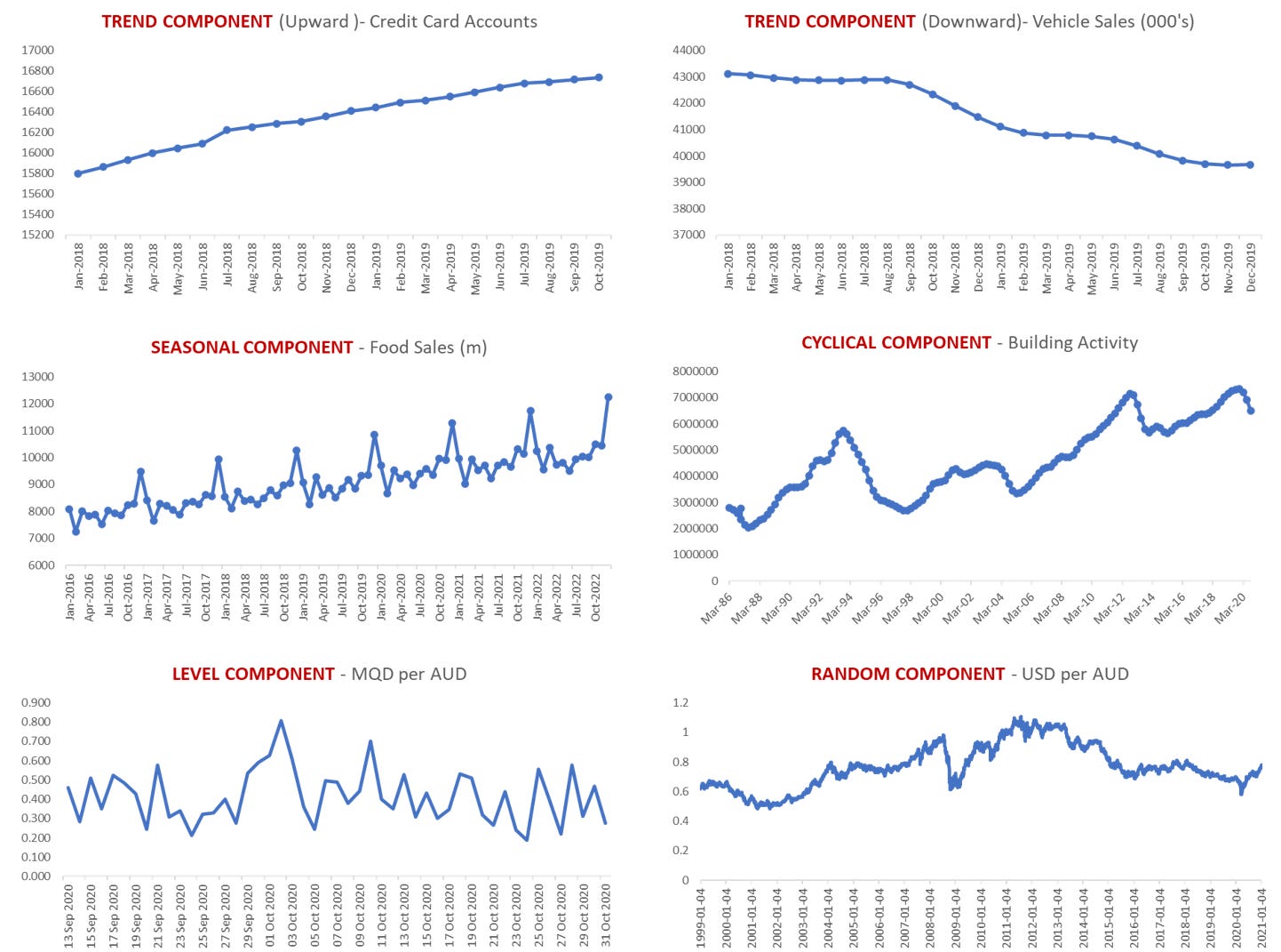
It's important to know what systematic component our data exhibits because that influences our choice of business forecasting methods.
Residual / Error Functions
Accuracy check of models is via error functions. The error functions are usually based on either the absolute errors or the squared errors due to the misleading interpretation of the average of errors.
There are many error functions and no one function is best. A good forecaster will use several functions as indicators of forecast performance of models. Sometimes the functions will differ in their choice of best model. The forecaster then must use other criteria to decide the preferred model.
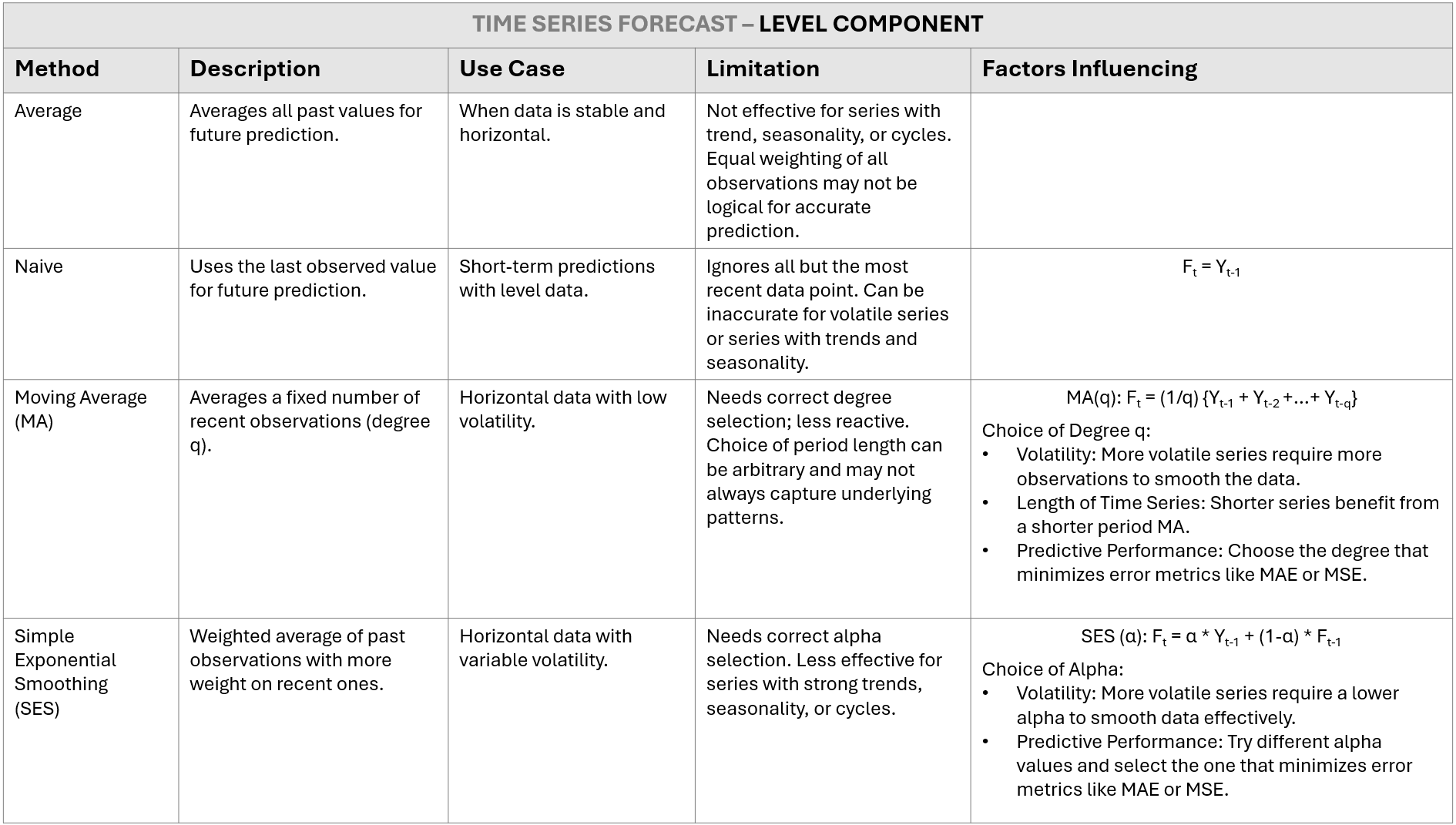
LEVEL COMPONENT TIME SERIES
Example Step-by-Step
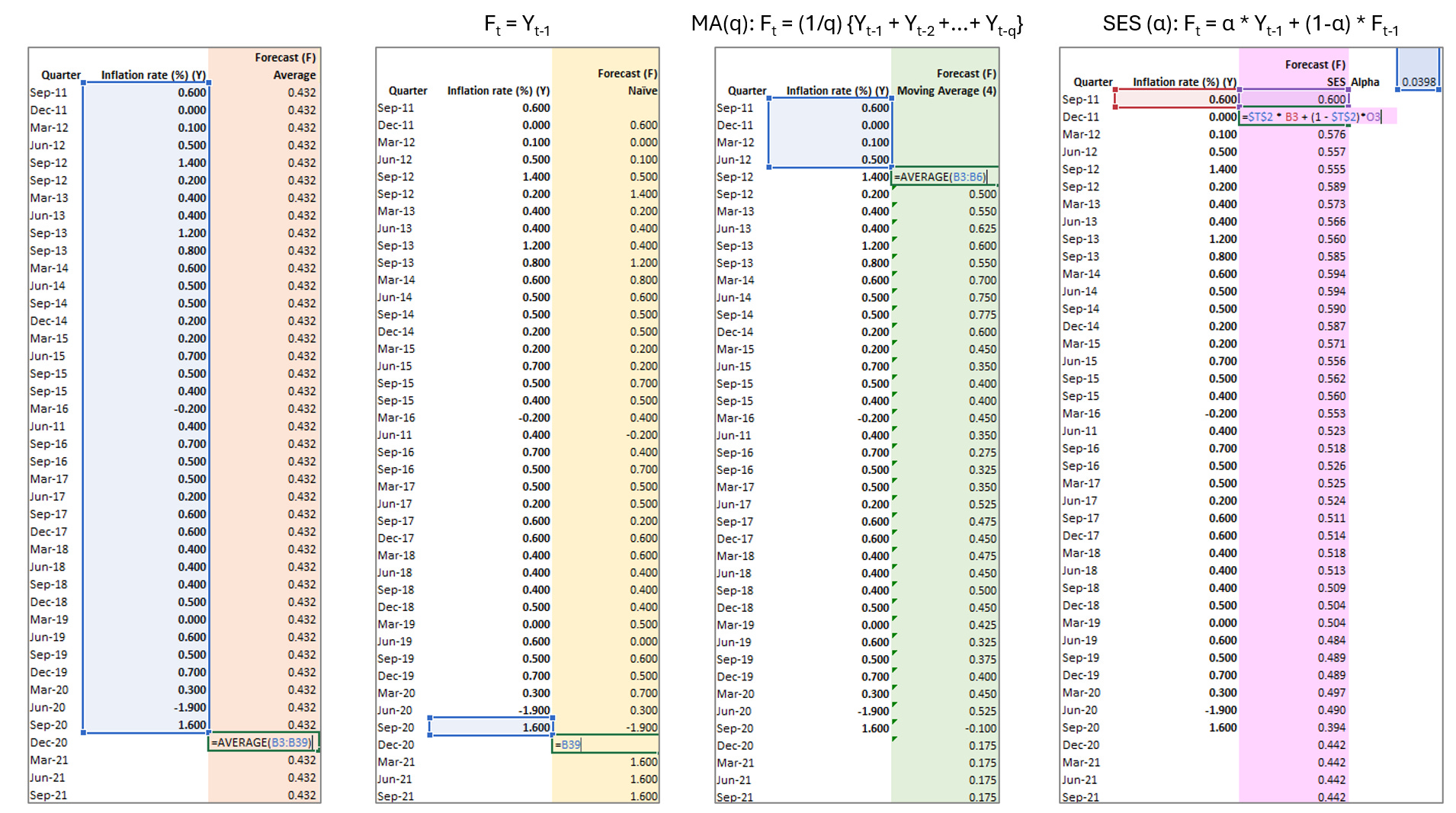

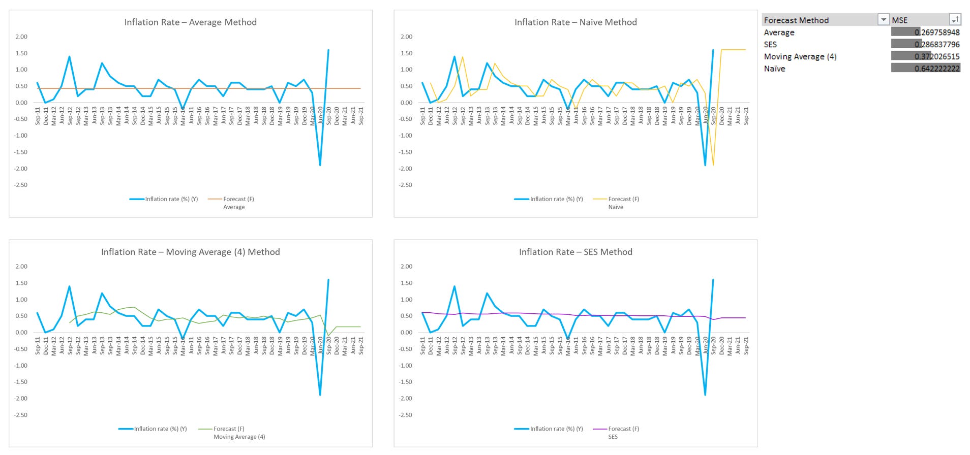
Example Result
Notes:
The naive forecast method is the simplest form of forecasting. It assumes that the demand for the current period will be the same as the previous period. You can adapt this method to your analysis context:
Seasonal Naive Method: For seasonal demand, use the same period from the previous year. For instance, the forecast for January this year would be the demand from January last year.
Growth Adjustment: If there is consistent growth, you can add a fixed amount (TTT) to account for the growth. Ft = Yt−1 + T
The naive method serves as a useful benchmark. Comparing it to more complex methods helps determine if those methods offer significant improvements in accuracy.
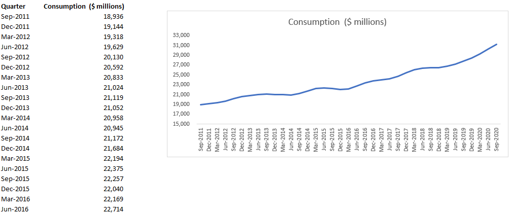
TREND COMPONENT TIME SERIES
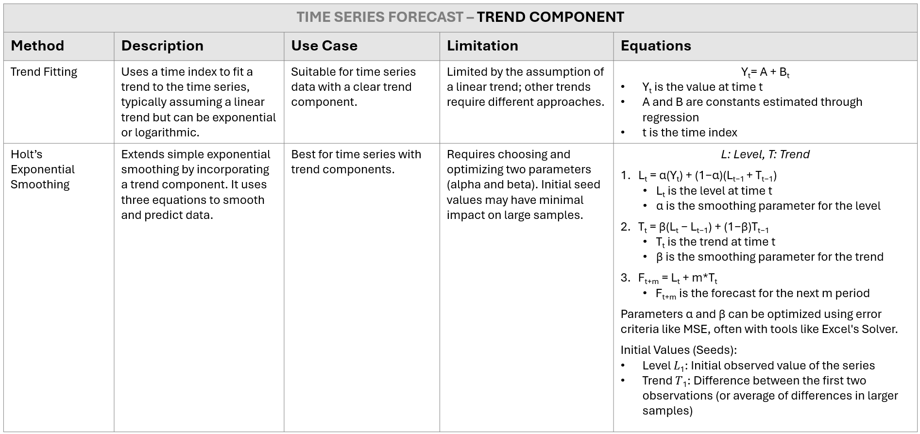
Trend Fitting Method
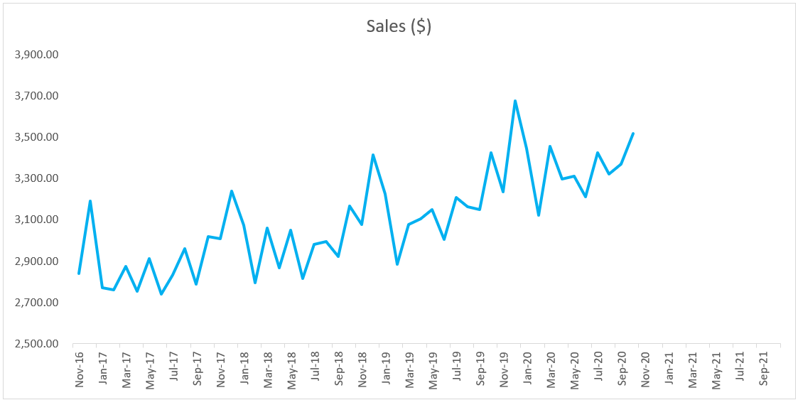
Step 1: Create Line chart
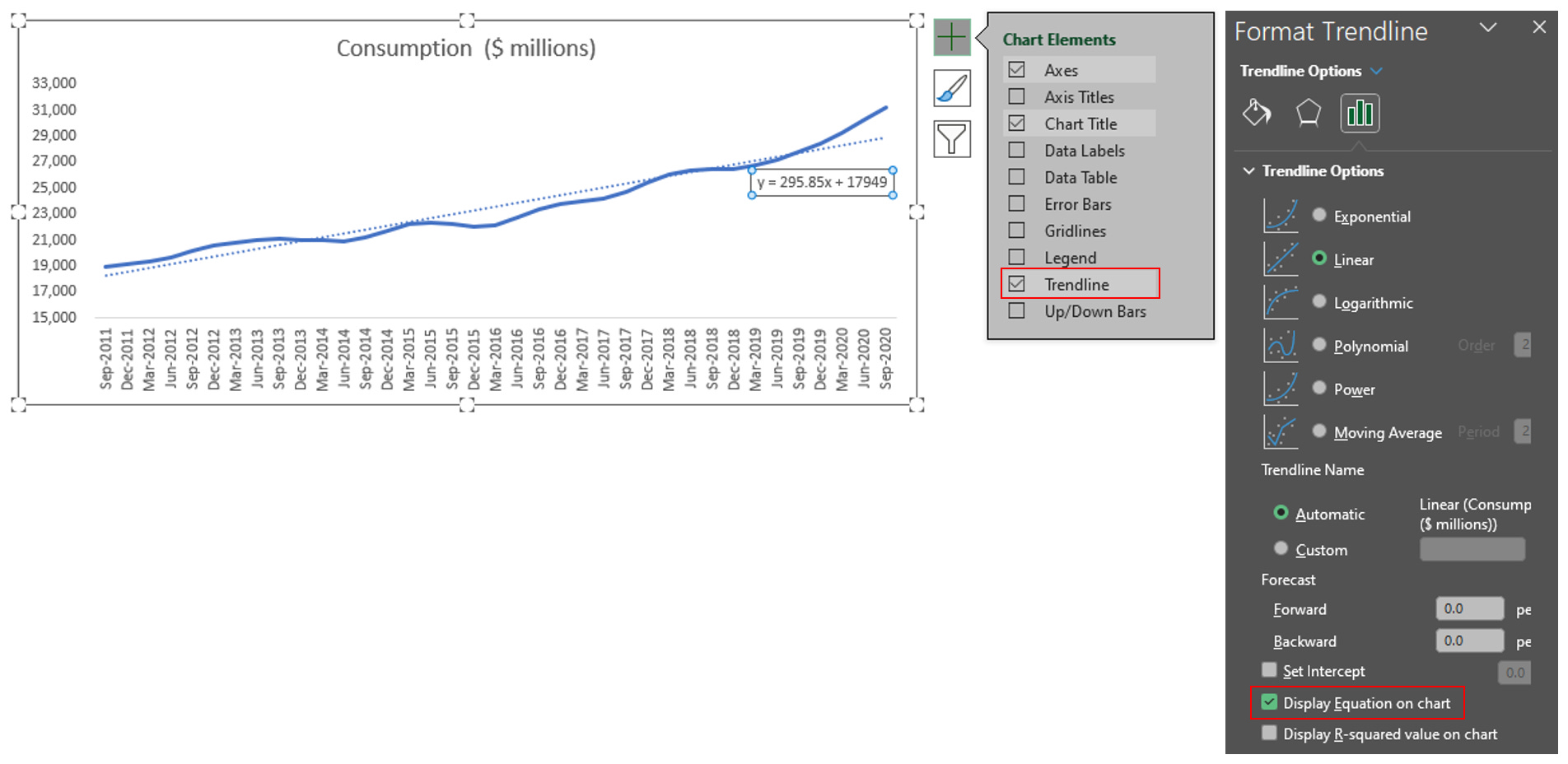
Step 2: Insert Trend line and Equation
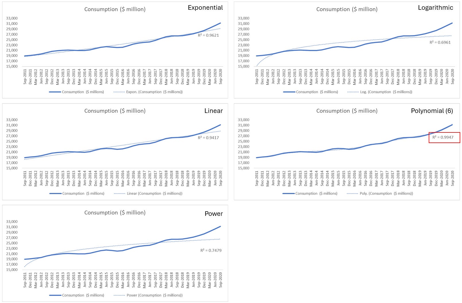
Step 3 (Optional): Choose the most suitable trendline options via R-squared value
Rule: You'd like the trendline that have R-squared number to be as close to one as possible.
In this example, we see that Polynomial with order 6 has the highest R-Squared. However the equation is pretty complicated for us to apply. So in the next step, I apply equation from Exponential and Linear trendline.
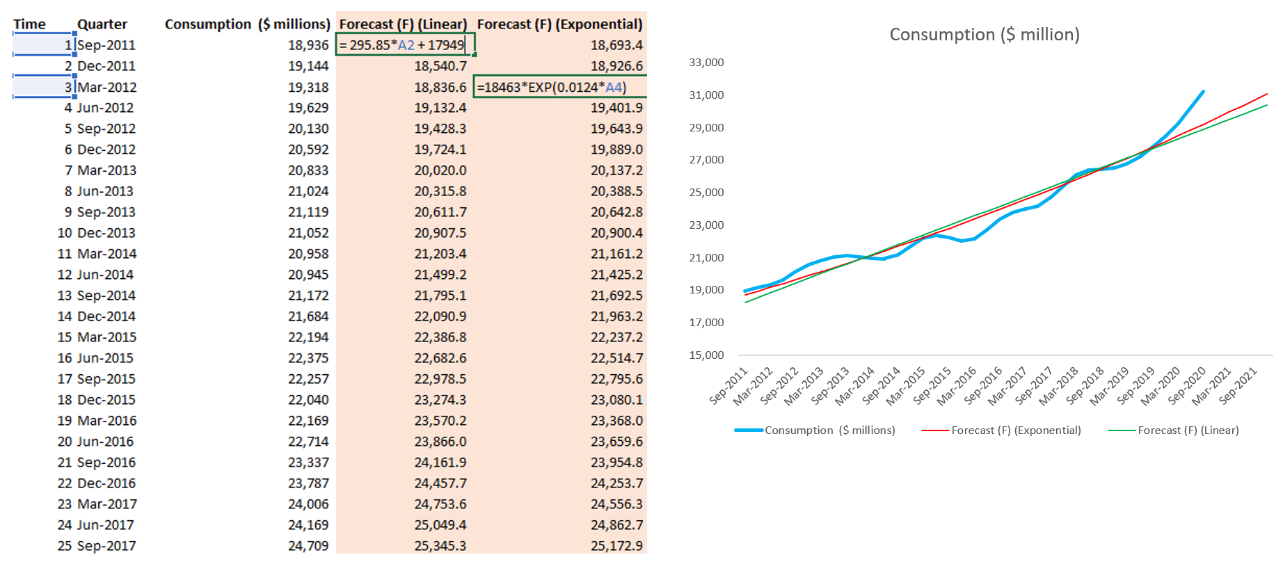
Step 4: Create Time column, copy equation from Exponential / Line chart and apply that formula to Forecast column
Holt’s Exponential Smoothing Method
Step 1: Create Line chart and Determine seeders of Level and Trend columns
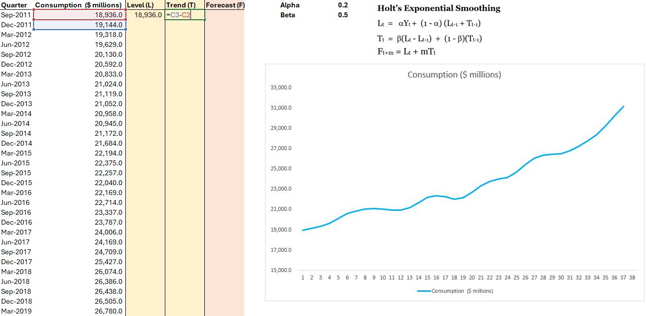
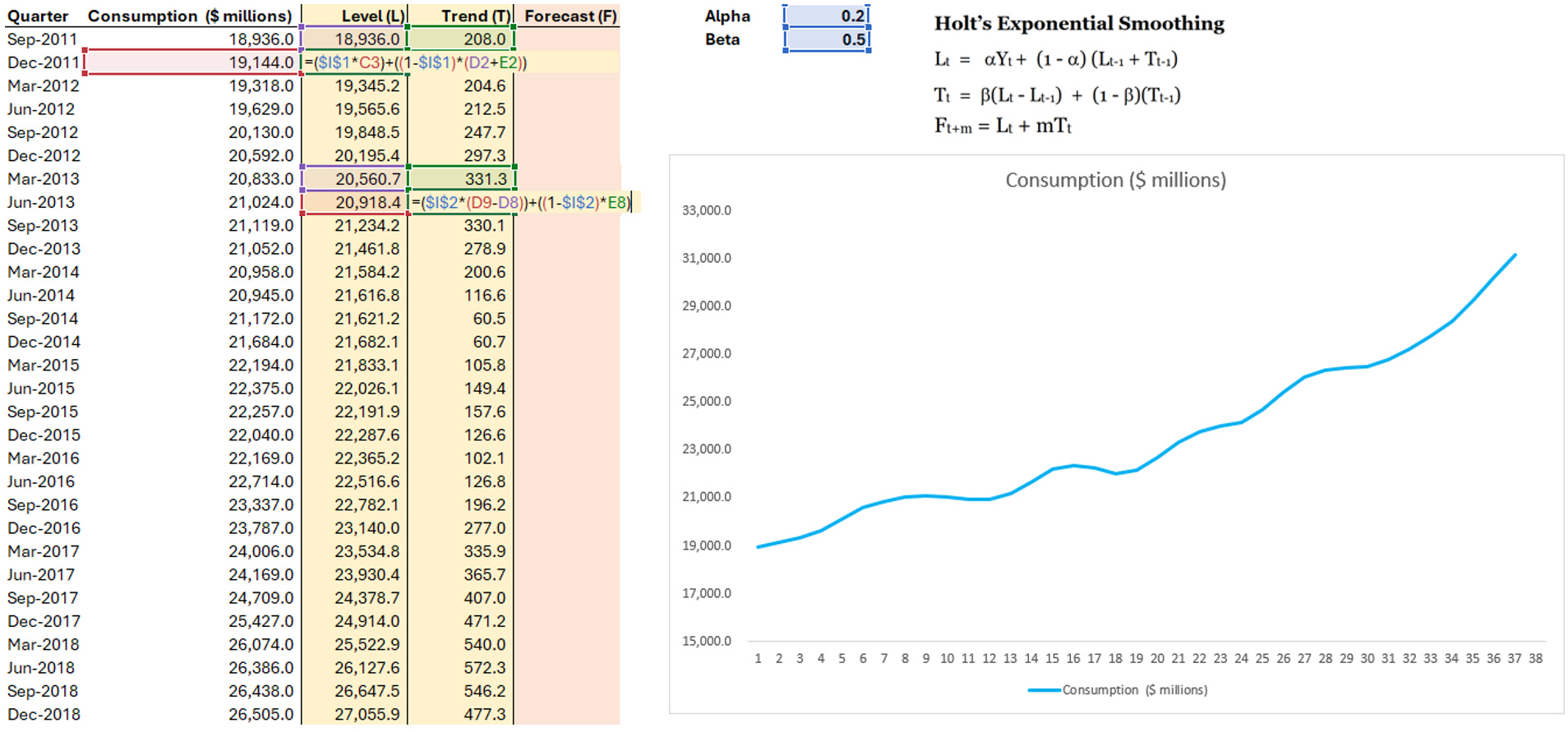
Step 2: Calculate Level and Trend column, follow the equation
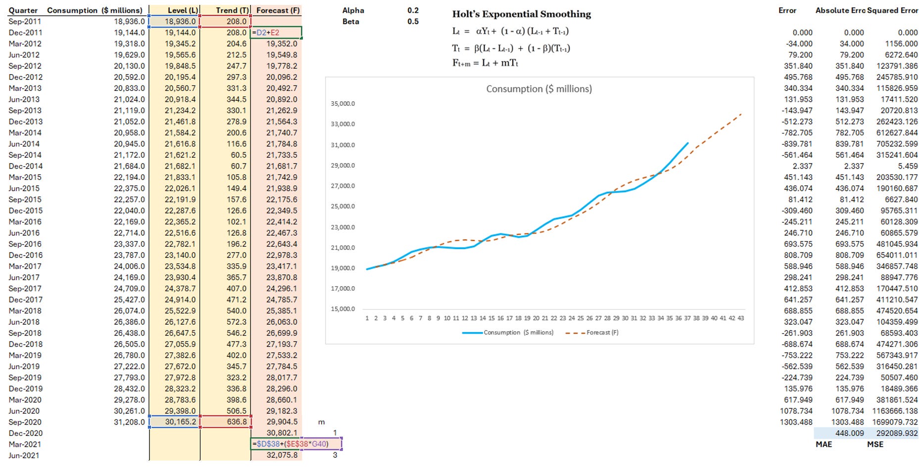
Step 3: Calculate Forecast column and MSE
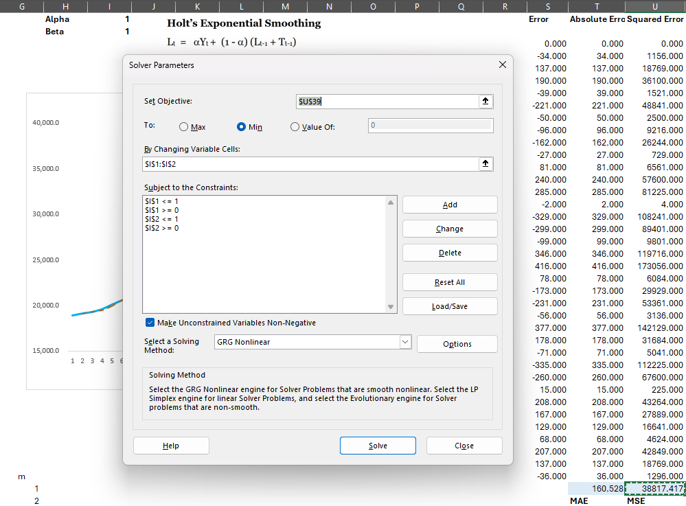
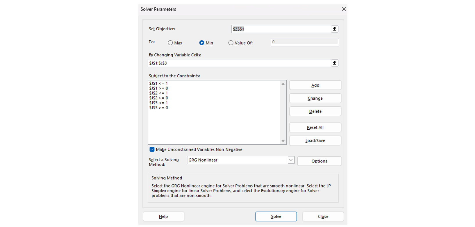
Step 4: Apply Solver to find Alpha and Beta values that lead to the lowest MSE
SEASONAL COMPONENT TIME SERIES
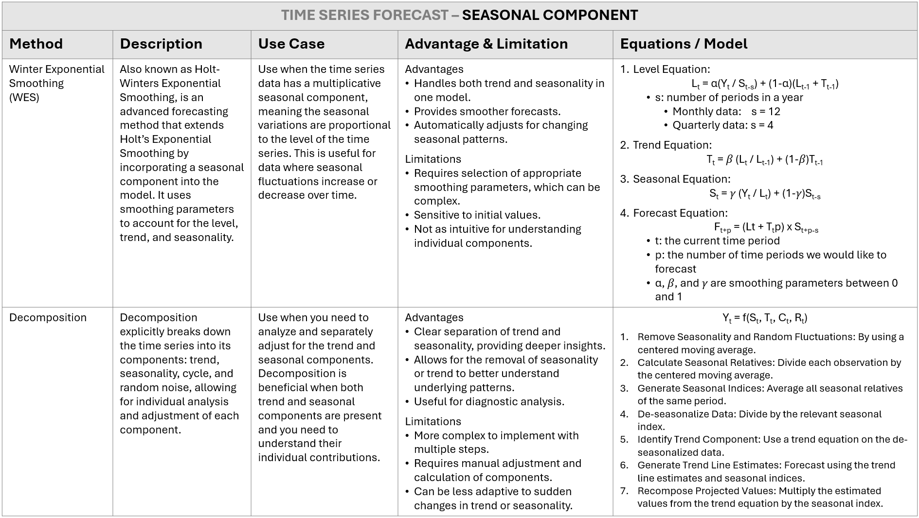
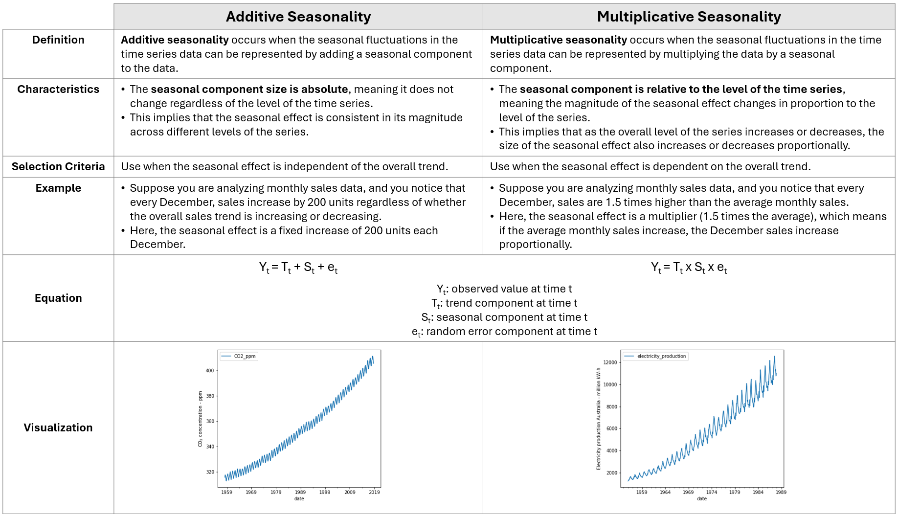
Broad Types of Seasonality
Seasonality can be classified into two broad categories.
Winter Exponential Smoothing (WES) - Multiplicative
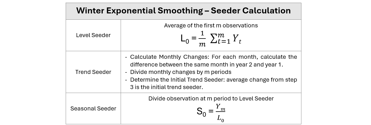
Step 1: Create Line chart and Determine seeders of level, trend, and seasonal column.
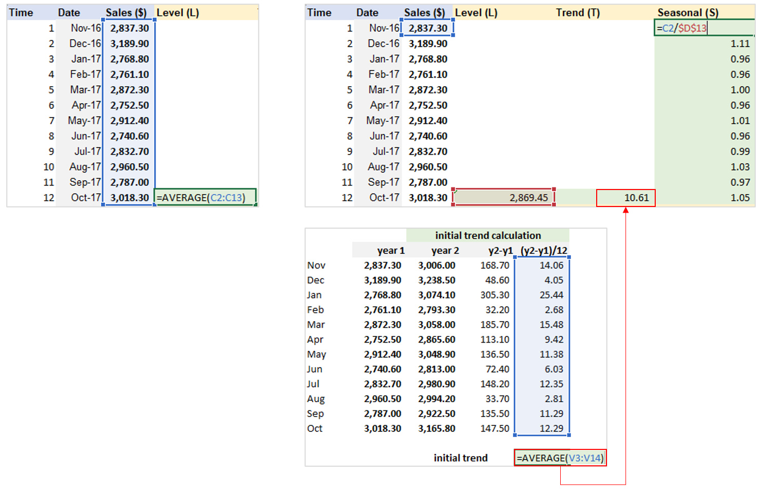
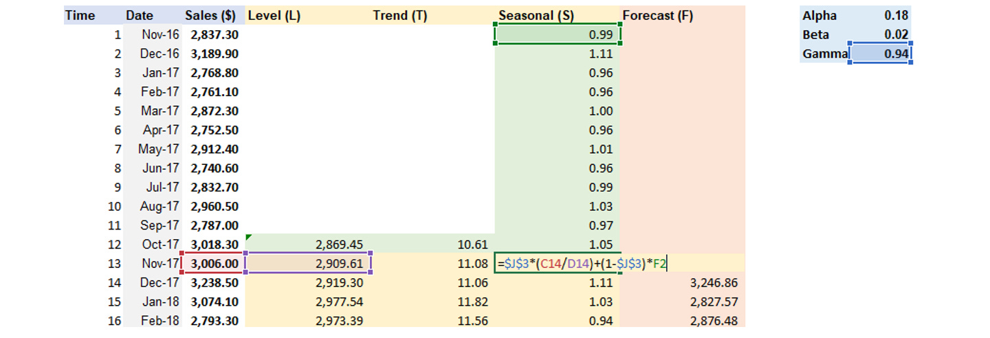
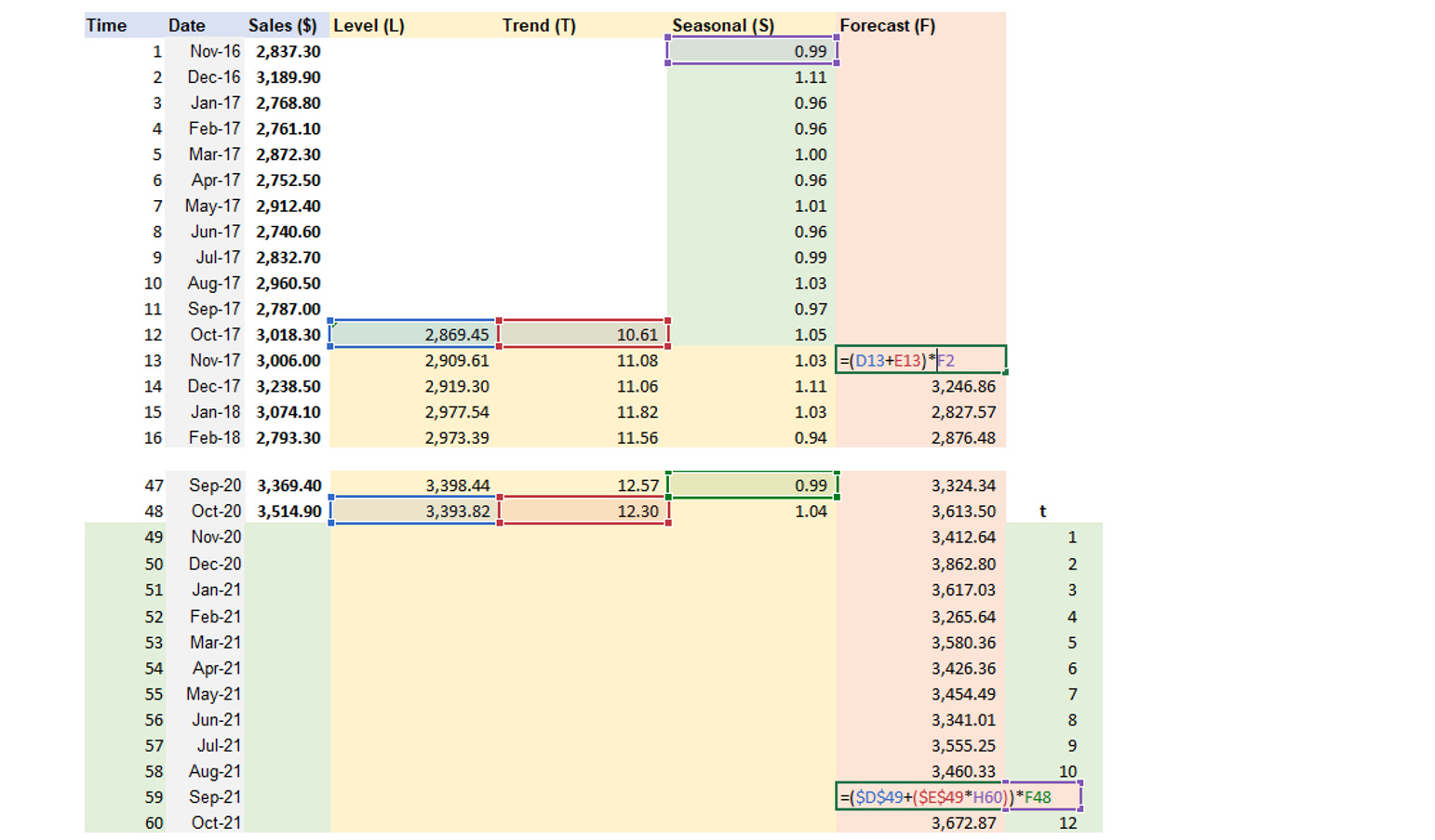
Step 2: Calculate Level, Trend, Seasonal components and Forecast
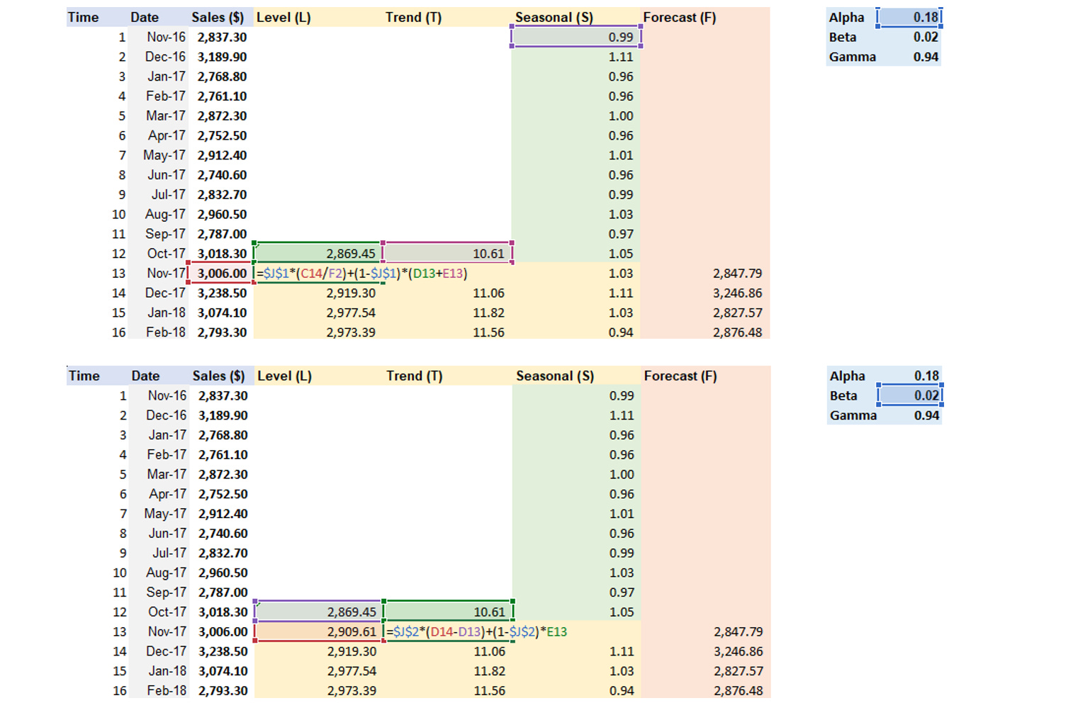
Step 3: Apply Solver to find Alpha, Beta, Gamma values that lead to the lowest MSE
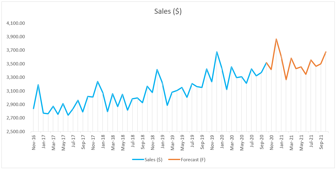
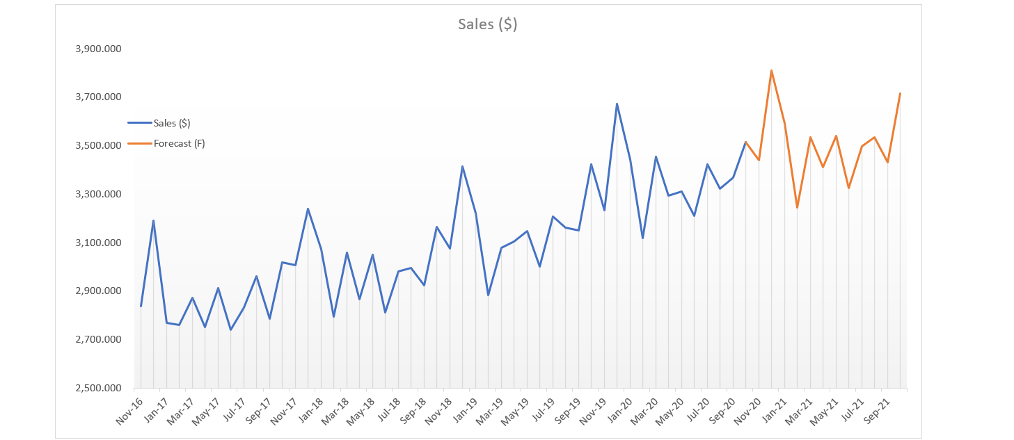
Step 4: Visualize forecast line in the chart
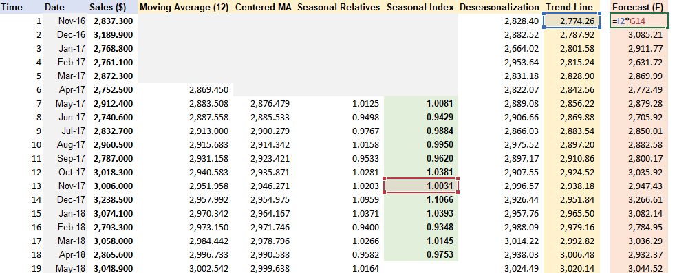
Decomposition - Multiplicative
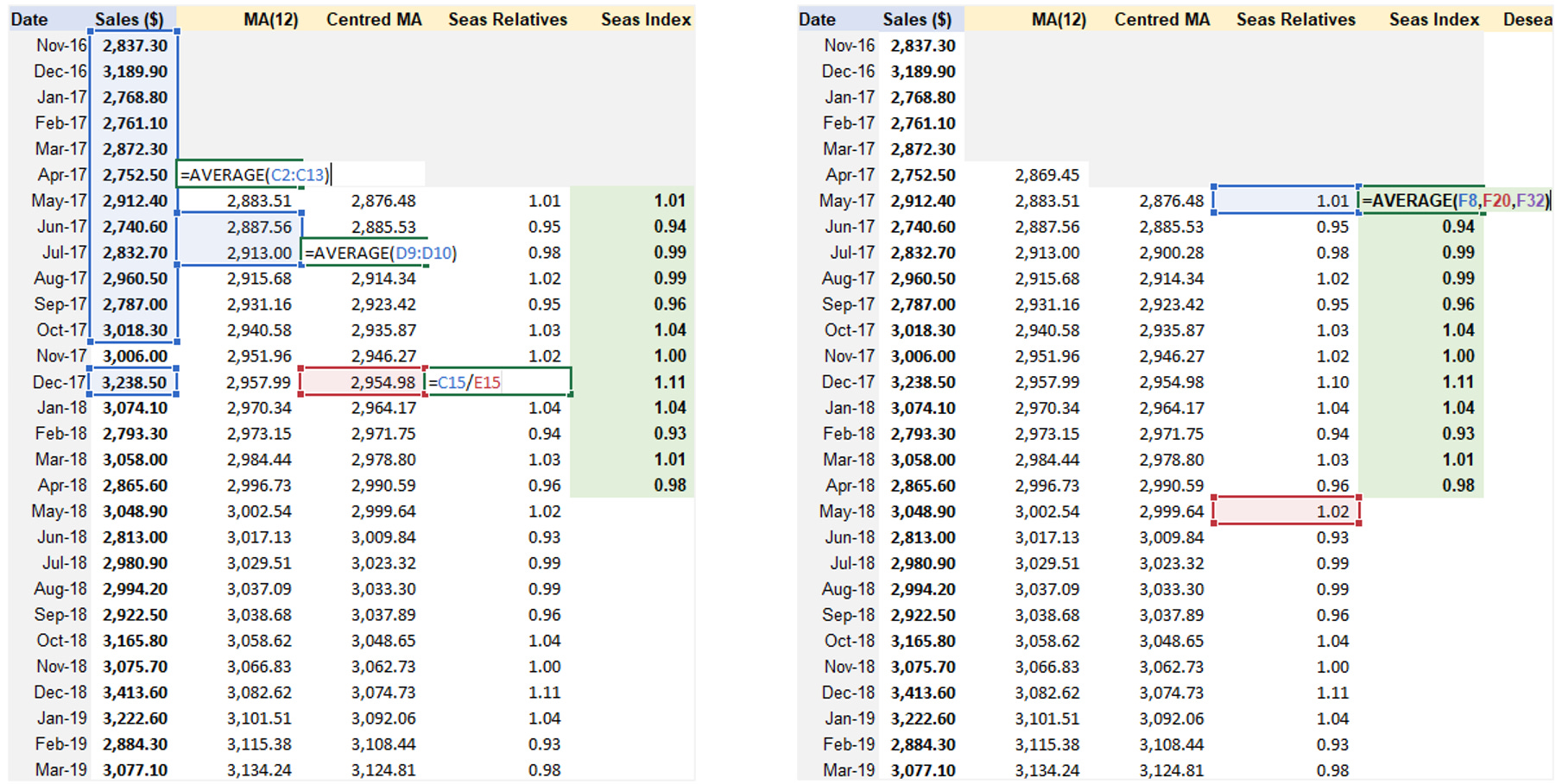
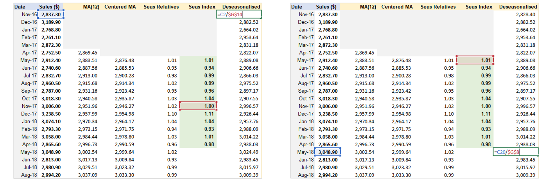
Step 1: Removing Seasonality & Random Variation + Seasonal Index Estimation.
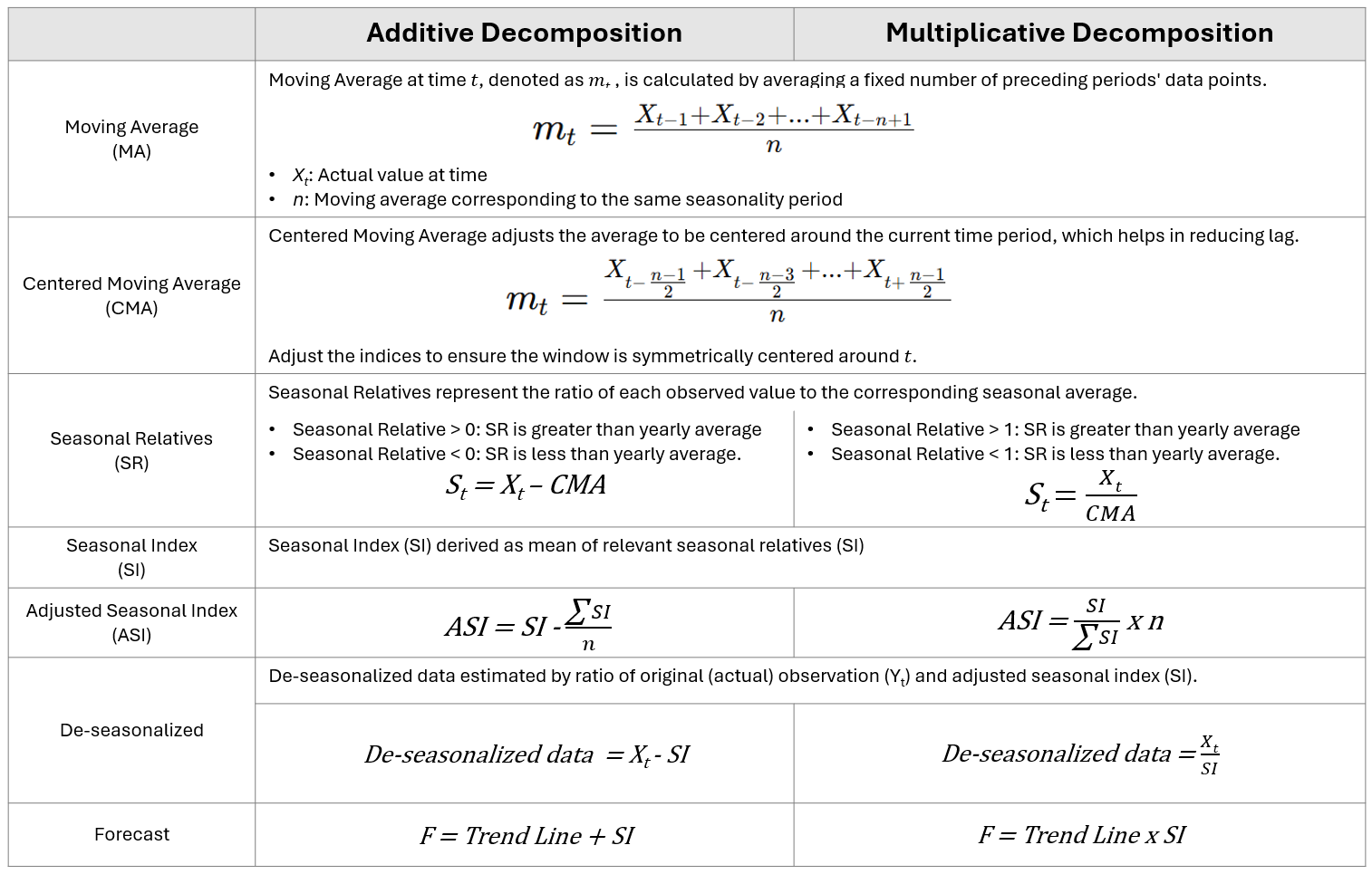
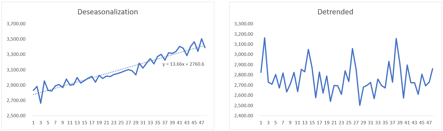
Step 2: De-seasonalize Data and Create Line Chart
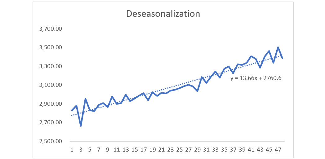
Step 3: Cycle & Trend separation
Insert variable t for time. Copy formula of trendline from De-seasonalization Chart and apply to Trend Line column, with x = time t.
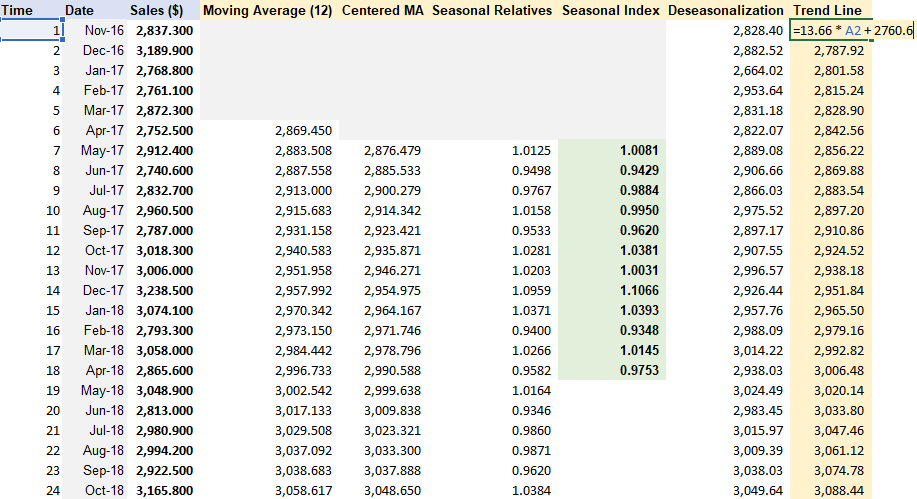
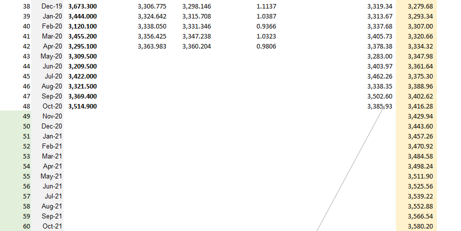
Step 4: Forecasting
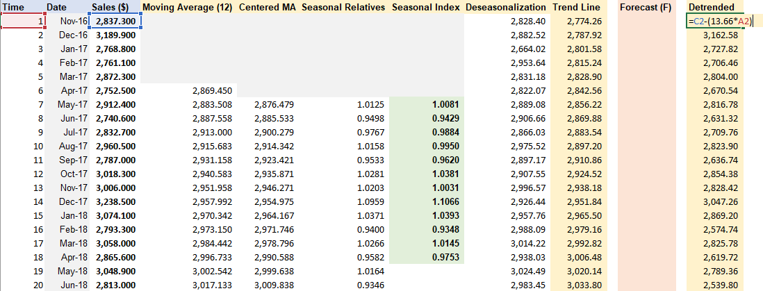
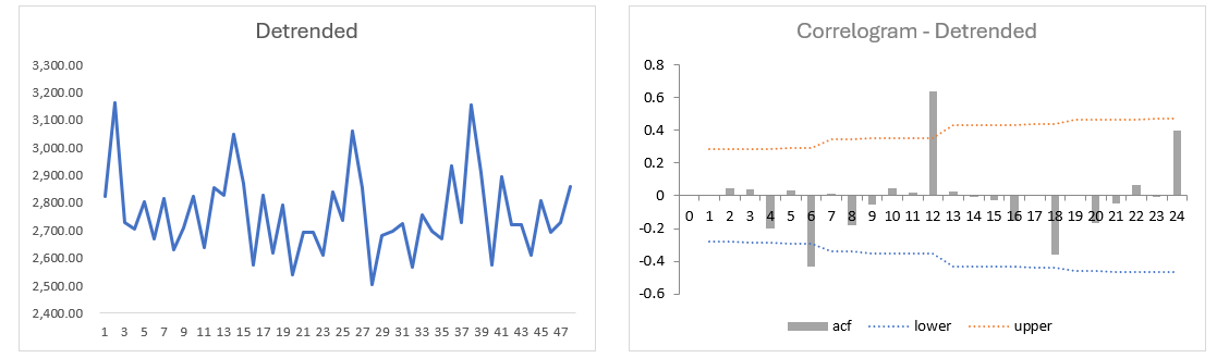
Step 5 (Optional): Detrended Data
Apply the same formula from trendline of De-seasonalization Data.
Detrended = Observation - slope x time t
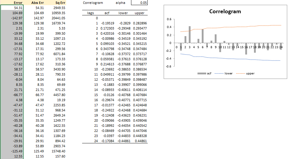
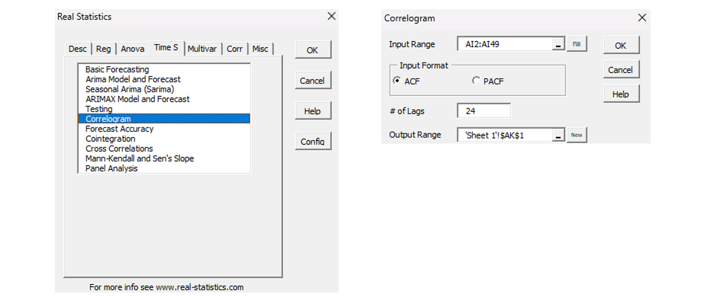
Step 6: Apply correlograms to validate error
Error criteria: (1) as small as possible, (2) should be random.
We observe that all those autocorrelation functions lie between the upper and lower bound and none of them cross the actual boundary except for the 3rd lag. We have evidence that our errors are fairly random, but there is that one issue with the third lag.
Step 7 (optional): Determine whether data has a trend component and whether data has a random component.
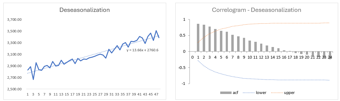
Create correlogram for “De-seasonalized Data” to determine whether data has a trend component.
those ACFs are slowly decreasing, then you've got evidence that there is in fact a trend component in your dataset
Create correlogram for “De-trended Data” to determine whether data has a seasonal component.
We can see those spikes in the ACF where it goes beyond the upper and lower bound, it's going outside that range, it happens to be the 6th, 12th, 18th, and 24th lag. It's happening at every six period intervals. That's a hint of regular periodicity. In other words, there is evidence of a seasonal component in data.
FAQs
Why we should calculate detrend and de-seasonalization data?
Detrending and deseasonalization are important steps in time series analysis and forecasting for several reasons. These processes help in isolating different components of the time series, which provides valuable insights and aids in building more accurate forecasting models.
Improved Forecasting Accuracy:
Detrending: Removes long-term trends to focus on other components such as seasonality and noise. This helps in identifying underlying patterns more clearly.
De-seasonalization: Removes seasonal effects to better understand the non-seasonal movements of the series. This allows for more accurate trend and cycle analysis.
Model Simplification: Simplifies the data, making it easier to model and analyze. It’s often easier to model a series with only one component (e.g., trend, seasonality) at a time.
Component Analysis: Helps in separately analyzing the trend, seasonal, and residual components. This can provide insights into how each component affects the overall time series.
Data Cleaning: Helps in identifying and removing anomalies and outliers that could be masked by trends or seasonality.
What insights can we get from it?
Understanding Long-term Trends: Detrending allows us to see the underlying growth or decline in the data over time. This is useful for strategic planning and understanding fundamental changes in the dataset.
Identifying Seasonal Patterns: Deseasonalization reveals the true nature of seasonal patterns. This helps in planning for recurring events and understanding the impact of seasonality on the data.
Isolating Cyclical Effects: By removing trend and seasonality, we can better identify cyclical effects which are important for economic and business cycle analysis.
Residual Analysis: The residual component, obtained after removing trend and seasonality, can be analyzed for randomness. This helps in validating the model. If the residuals are purely random, the model is good. If not, there might be other underlying patterns that need to be modeled.
Enhanced Predictive Models: By working with detrended and deseasonalized data, forecasting models can be more accurate as they can focus on the remaining components without interference from trends or seasonality.
Example: Consider a retail business analyzing monthly sales data. The data shows a clear upward trend due to business expansion and strong seasonal spikes in December.
Detrending: By removing the upward trend, the business can focus on understanding seasonal effects and random variations. This can reveal whether sales are truly increasing due to business activities or just due to trend.
Deseasonalization: By removing the seasonal spikes, the business can better understand the underlying trend and cyclical behaviors. This can help in inventory planning, staffing, and understanding the impact of promotional activities.
Why error should be as small as possible and random?
Errors Should Be As Small As Possible
Accuracy: (1) Small errors indicate forecasts are close to actual values, capturing underlying patterns. (2) High accuracy improves decision-making and planning, reducing costly errors.
Performance: Smaller errors reflect superior model performance.
Confidence: Low error rates increase confidence in forecasts. Stakeholders trust models that consistently produce small errors.
Errors Should Be Random:
Model Completeness: Random errors show the model captures all systematic patterns like trends, seasonality, and cycles. Non-random errors suggest that there are still patterns in the data that the model has not accounted for, indicating an incomplete or inadequate model.
Bias-Free Forecasts: Random errors mean forecasts are unbiased, with errors equally likely to be positive or negative. Non-random errors (bias) mean the model consistently overestimates or underestimates values.
Predictive Validity: Random errors suggest high predictive validity, allowing generalization to new data. Non-random errors may indicate overfitting, capturing noise instead of true patterns.
Diagnosis and Improvement: Randomness analysis helps diagnose model issues.
Non-random errors require further investigation to correct model deficiencies, such as missing variables or incorrect assumptions.
What is correlogram? What does lags mean?
What is a Correlogram?
A correlogram is a graphical tool used in time series analysis. It shows the relationship between a time series and its past values (lags).
It helps identify patterns like trends, seasonality, and randomness in the data.
Why Use a Correlogram?
To check if your model has captured all patterns.
To identify if any systematic patterns (like trends or seasonality) remain.
To ensure that the errors in your forecasting model are random and not patterned.
What are Lags? The time difference between a value in the time series and a past value. Example: If you have monthly sales data, a lag of 1 means comparing this month’s sales to last month’s sales.
Understanding the Correlogram:
X-axis (Horizontal): Represents different lag times (e.g., 1 month, 2 months, etc.).
Y-axis (Vertical): Represents the correlation coefficient, showing how much a past value (lag) influences the current value.
Correlation Coefficient: Ranges from -1 to 1.
+1: Perfect positive correlation (as one value increases, the other also increases).
-1: Perfect negative correlation (as one value increases, the other decreases).
0: No correlation.
Interpreting a Correlogram:
Significant Spikes:
Spikes outside the confidence bounds indicate significant correlation at that lag.
These spikes suggest patterns in the data.
Confidence Bounds:
Bounds around the y-axis (usually dashed lines) to judge if correlations are significant.
Spikes within bounds suggest random noise; spikes outside bounds indicate patterns.
Pattern Recognition:
Trend: Slowly decreasing correlation over lags.
Seasonality: Regular spikes at specific lags (e.g., every 12 months for annual seasonality).
Mastering time series forecasting involves understanding diverse methods like moving averages and more complicated models. These tools not only predict future trends but also empower data-driven decision-making across industries. Be noted, this is just the basic of Time Series Forecasting; spending more time to explore advanced models is necessary to unlock deeper insights and refine predictive accuracy.